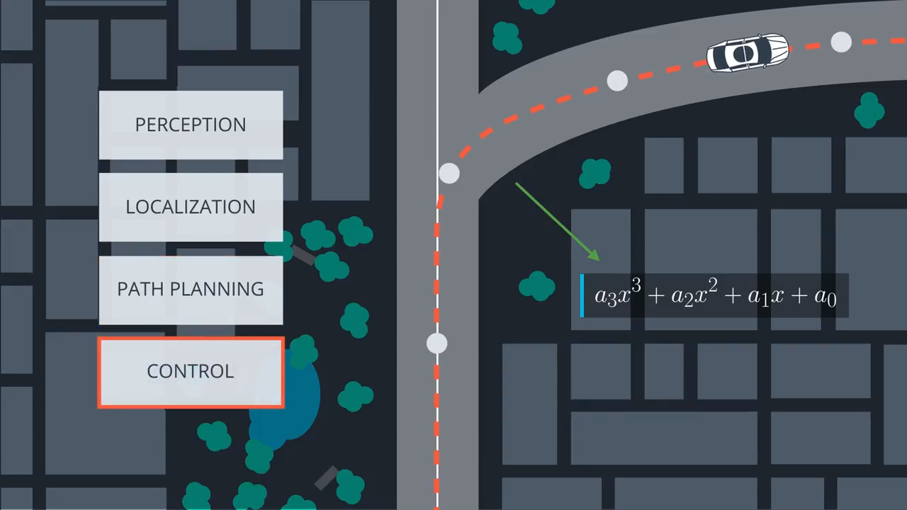
Autonomous vehicle system architecture starts with the perception system, which estimates the state of the surrounding environment including landmarks and vehicles and pedestrians.
The localization block compares a model to a map to figure out where the vehicle is.
The path planning block charts a trajectory using environmental model, the map and vehicle location.
Finally, the control loop applies the actuators to follow this trajectory.
Typically, the path planning block passes the reference trajectory to the control block as a polynomial. Third degree polynomials are common so they can fit most roads.
Fitting polynomials

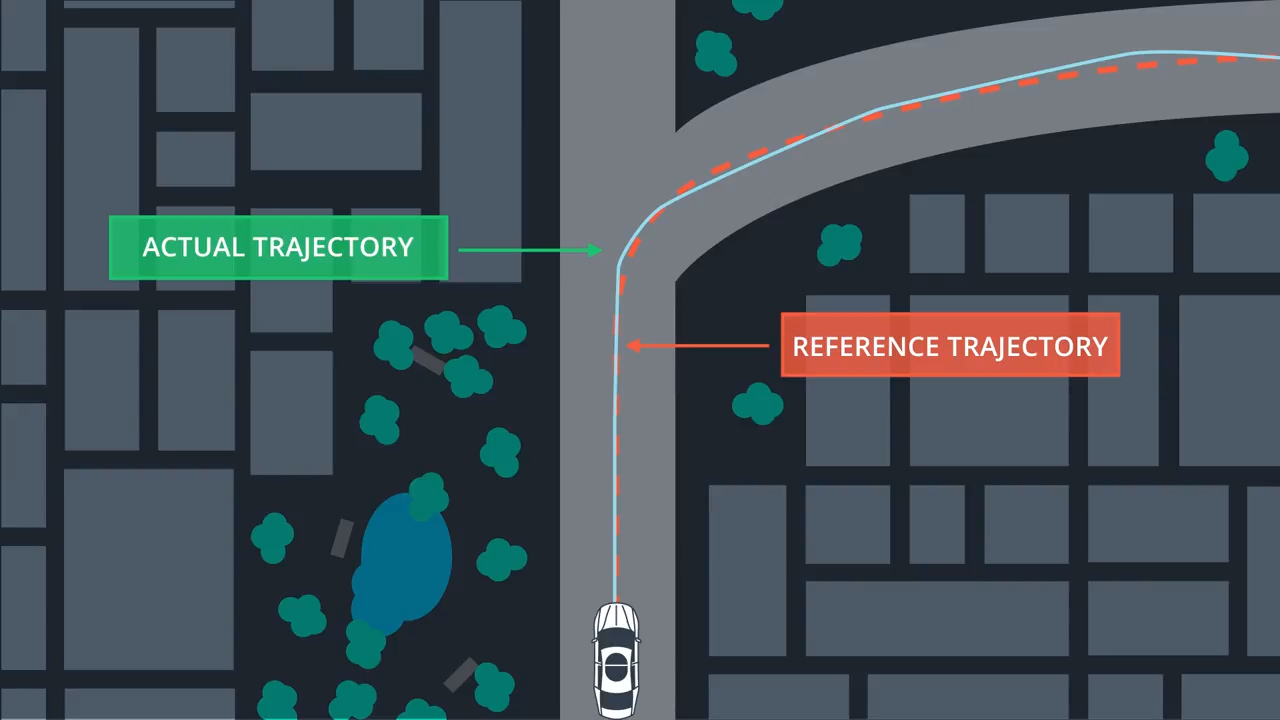
A controller actuates the vehicle to follow the reference trajectory within a set of design requirements. One important requirement is to minimize the area between the reference trajectory and the vehicle’s actual path. This error can be minimized by predicting the vehicle’s actual path and then adjusting the control inputs to minimize the difference between that prediction and the reference trajectory. The vehicle’s future states can be predicted by a kinematic model.
Once the predicted error is calculated by comparing the predicted path with the reference trajectory the vehicle can be actuated to minimize the error over time.
Errors
To follow a trajectory we want to minimize the predicted distance of the vehicle from the trajectory. This deviation is also known as the cross track error ($cte$). We also want to minimize the predicted difference, or angle, between the vehicle orientation and trajectory orientation. We’ll call this the psi error ($e\psi$). The required desired orientation can be calculated as the tangential angle $\psi_{des}$ of the reference trajectory (polynomial).
While we might wish to set the speed to a reference, i.e. 35 mph, the speed itself is not something we want to minimize. Otherwise we’d end up minimizing the speed below zero and driving in reverse.


Comments