Mathematics - Linear Algebra

Introduction

The following sections introduce some topics of linear algebra. For more mathematical topics checkout other list. Linear algebra can be used to describe the manipulation of space through the use of transformation matrices, which is used in computer graphics and robotics. It also lets us solve systems of equations.

Vectors

Span, Bases and Linear Combinations

The span of two vectors $\vec{v}$ and $\vec{w}$ is the set of all their linear combinations. $$ a\vec{v}+b\vec{w} $$ where $a$ and $b$ varay over all real numbers $\mathbb{R}$.

Vectors are said to be linearly independent if $$ \vec{u} \neq a\vec{v}+b\vec{w} $$ for all values $a$ and $b$. Otherwise they are linearly dependent if one vector can be expressed in terms of the others $$ \vec{u} = a\vec{v}+b\vec{w} $$

The basis of a vector space is a set of linearly independent vectors that span the full space

Matrices as Linear Transformations

Important topic in linear algebra that shows the relation between linear transformations (can be seen as a funciton $f(x)$) and matrices. Usually such linear transformations transform one vector $\vec{v}$ to another vector $\vec{w} = L(\vec{v})$.

Given a basis with vectors $\hat{i} = \begin{bmatrix}1 & 0 \end{bmatrix}$ and $\hat{j} = \begin{bmatrix}0 & 1 \end{bmatrix}$ that span the 2D space, matrices can be thought of as transformations of that space. In a given matrix

\[\begin{bmatrix} a & c \\ b & d \end{bmatrix}\]

with respect to the original basis, the first matrix column tells us where the first basis vector $\hat{i}$ lands (or gets transformed to) and the second column shows where the basis vector $\vec{j}$ lands in that linear transformation.

A linear transformation is linear if it has two properties: - All lines must remain lines (without getting curved) - Origin must remain fixed in place which means that grid lines must remain parallel and evenly spaced.

To program a transformation function numerically, it is only necessary to record where the basis vectors $\hat{i}$ and $\hat{j}$ each land. With this information, other vectors can be transformed using these transformed basis vectors as columns in a new transformation matrix. An arbitrary vector $\vec{v}$ can then be transformed by that matrix. This can be seen as scaling the transformed basis vectors by the vector components of $\vec{v}$ or as one specific linear combination. $$ \begin{bmatrix} i_x & j_x \\ i_y & j_y \end{bmatrix} \begin{bmatrix} v_x \\ v_y \end{bmatrix} = \underbrace{ v_x \begin{bmatrix} i_x \\ i_y \end{bmatrix} + v_y \begin{bmatrix} j_x \\ j_y \end{bmatrix}}_{\text{Where all the intuition is}} = \begin{bmatrix} i_x v_x & j_x v_y \\ i_y v_x & j_y v_y \end{bmatrix} $$

Matrix Multiplication as Composition

Three Dimensional Linear Transformations

Transformations in three dimensions work just like transformations in two dimensions only with three dimensional vectors as input and output and three by three transformation matrices.

$$ \vec{v} = \begin{bmatrix} x_i \\ y_i \\ z_i \\ \end{bmatrix} \rightarrow L(\vec{v}) \rightarrow \begin{bmatrix} x_o \\ y_o \\ z_o \\ \end{bmatrix} = \vec{w} $$

As in two dimensions, a three dimensional transformation is completely described by where the three unit basis vectors $\hat{i}$, $\hat{j}$, $\hat{k}$ go. Given a three dimensional transformation matrix, the output coordinates of the basis vectors are given by the matrix columns. Transforming a three dimensional input vector can be thought of scaling each basis vector with the corresponding input coordinate, which results in the transformed output vector.

$$ \vec{w} = L(\vec{v}) = \begin{bmatrix} \vert & \vert & \vert \\ \hat{i} & \hat{j} & \hat{k} \\ \vert & \vert & \vert \\ \end{bmatrix} \begin{bmatrix} x \\ y \\ z \\ \end{bmatrix} = x \hat{i} + y \hat{j} + z \hat{k} $$

The Determinant

The determinant of a matrix is the factor by which a given area, for example the unit square, increases or decreases after applying the transformation matrix.

The scaling factor by which a linear transformation changes any area is called the determinant of that transformation.

If the determinant is zero $\text{det}(M) = 0$ a two dimensional area is squished onto a line or even a single point when given for example the zero matrix.

Negative determinant values $\text{det}(M) < 0$ describe a transformations that invert the orientation of space or put differently: flipping the space over. In terms of basis vectors it means that the $L(\hat{i})$ is to the left of $L(\hat{j})$ after a transformation $L$, where before the transformation $\hat{j}$ is to the left of $\hat{i}$. However, the absolute value of the determinant tells us about the factor about which the area has been scaled after applying the transformation.

In three dimensions the determinant tells us how much volume gets scaled. A one by one by one cube resting on the basis vectors $\hat{i}$, $\hat{j}$, $\hat{k}$ gets warped into a parallelepiped after applying a transformation. The same two dimensional flipping concept is true for three dimensions, where the right hand rule comes into play. $\hat{i}$ goes into the direction of the forefinger, the middle finger points in a right angle from $\hat{i}$ and is defined as $\hat{j}$ and finally the thumb points upwards and defines $\hat{k}$. After this finger combination is possible after a transformation, the determinant is positive and the orientation has therefore not changed. Otherwise the determinant is negative and we could apply the left hand rule.

A determinant of zero means that the columns of the matrix are linearly dependent.

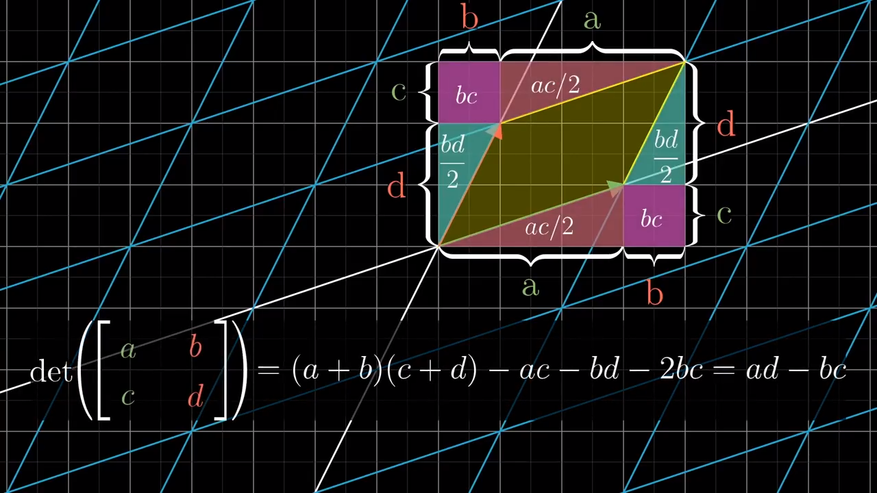
To compute the determinant of a two by two matrix we apply the following rule:

$$ \text{det} \begin{bmatrix} a & b \\ c & d \\ \end{bmatrix} = ad - bc $$

For three dimensional matrices the determinant is

$$ \text{det} \begin{bmatrix} \color{green}{a} & \color{red}{b} & \color{blue}{c} \\ \color{green}{d} & \color{red}{e} & \color{blue}{f} \\ \color{green}{g} & \color{red}{h} & \color{blue}{i} \\ \end{bmatrix} = \color{green}{a} \text{det} \begin{bmatrix} \color{red}{e} & \color{blue}{f} \\ \color{red}{h} & \color{blue}{i} \\ \end{bmatrix} - \color{red}{b} \text{det} \begin{bmatrix} \color{green}{d} & \color{blue}{f} \\ \color{green}{g} & \color{blue}{i} \\ \end{bmatrix} + \color{blue}{c} \text{det} \begin{bmatrix} \color{red}{e} & \color{red}{e} \\ \color{red}{h} & \color{red}{h} \\ \end{bmatrix} $$

Taking the determinant of a composition of two matrix transformations $\text{det}(M_1M_2)$ results in the product of the determinants of the single matrices. Intuitively this corresponds to applying multiple factors to each resulting area after each corresponding transformation.

$$ \text{det}(M_1M_2) = \text{det}(M_1)\text{det}(M_1) $$

Inverse Matrices, Column Space and Null Space

Gaussian elimination
Row echelon form

With linear algebra we can solve systems of equations with a list of unknown variables and a list of equations relating them. In linear algebra these variables get only scaled and added to each other but not modified by any other nonlinear function, for example squared, multiplied by each other, or the sine or cosine of that variables.

Nonsquare Matrices as Transformations between Spaces

With nonsquare matrices it is possible to transform between dimensions.

$$ \underbrace{\vec{v} = \begin{bmatrix} x_i \\ y_i \\ \end{bmatrix}}_{\text{2D vector}} \rightarrow L(\vec{v}) \rightarrow \underbrace{\begin{bmatrix} x_o \\ y_o \\ z_o \\ \end{bmatrix} = \vec{w}}_{\text{3D vector}} $$

Such transformations are also linear because the grid lines in the input and outputspace remain parallel and evenly spaced. Also the origin maps to the origin. The matrix columns describe where the basis vectors of the input space land (get transformed to) in the output space.

A $m \times n$ matrix $\mathbf{A}\in\mathbb{R}^{m\times n}$ has $m$ rows and $n$ columns which maps the $n$ dimensional input space (with its $n$ basis vectors) to the $m$ dimensional output space (which has $m$ basis vectors). The $m$ rows indicate that the landing spots for each of those $n$ basis vectors of the input is described with $m$ separate coordinates.

$$ \mathbf{A} \vec{v} = \begin{bmatrix} a_{11} & a_{12} & \cdots & a_{1n} \\ a_{21} & a_{22} & \cdots & a_{2n} \\ \vdots & \vdots & \ddots & \vdots \\ a_{m1} & a_{m2} & \cdots & a_{mn} \\ \end{bmatrix} \begin{bmatrix} v_1 \\ v_2 \\ \vdots \\ v_n \\ \end{bmatrix} = \begin{bmatrix} w_1 \\ w_2 \\ \vdots \\ w_m \\ \end{bmatrix} = \vec{w} $$

The column space of this matrix (also the span of the columns or space where all vectors land) $n$ dimensional space slicing through the origin of the $m$ dimensional space. For a $3\times 2$ matrix this would be a 2 dimensional plane slicing through the origin of the three dimensional plane.

Such a nonsquare matrix can still have full rank if the number of dimensions in the column space is equal to the number of dimensions of the input space.

Dot Product and Duality

Given two vectors $\vec{v}$ and $\vec{w}$ the dot product between them is defined as

$$ \vec{v} \cdot \vec{w} = v_1 w_1 + v_2 w_2 + \cdots + v_n w_n $$

which results in a single number. This means that the dot product can be interpredted as linear transformation that maps an $n$ dimensioanl vector the the one dimensional space (the number line).

Geometrically the dot product describes a projection of one vector onto another. It is defined as the length of the projected vector multiplied with the length of the vector that defines a line on which we projected the first vector. It is important to note that the dot product is commutative. Other properties are given by the angle between the two vectors:

If the angle $\theta$ is obtuse ($\theta > 90^\circ$) then the dot product is negative $\vec{v} \cdot \vec{w} < 0$
If the angle $\theta$ is acute ($\theta < 90^\circ$) then the dot product is positive $\vec{v} \cdot \vec{w} > 0$
The dot product is zero $\vec{v} \cdot \vec{w} = 0$ if the angle is straight ($\theta = 90\deg$)

Cross Product

The value of the cross product of two vectors $\vec{v}$ and $\vec{w}$ can be considered as the area of the parallelogram these vectors span. The calculation is done using the determinant which describes how the area of a linear transformation changes (resulting in the factor). In the definition below the two vectors describe a linear transformation of the basis vectors $\hat{i}$ and $\hat{j}$ which span the unit square and that has an area of one. After the transformation that square gets turned into the parallelogram which area is given in the formula below.

$$ \vec{v} \times \vec{w} = \text{det}\left( \begin{bmatrix} \vert & \vert \\ \vec{v} & \vec{w} \\ \vert & \vert \end{bmatrix} \right) $$

The sign of this area depends on the orientaiton of the parallelogram, which means that the order of the cross product matters.

If $\vec{v}$ is on the right of $\vec{w}$ then the result is positive and negative otherwise.
The more perpendicular the vectors are, the bigger the cross product gets.
$(a\cdot\vec{v})\times\vec{w} = a(\vec{v}\times\vec{w})$

The cross product defines a vector that is perpendicular to the the parallelogram with the resulting vector defined using the right hand rule.

$$ \vec{v} \times \vec{w} = \vec{p} $$

Cross Product in depth

$$ \vec{p} = \vec{v} \times \vec{w} = \text{det}\left( \begin{bmatrix} \hat{i} & v_1 & w_1 \\ \hat{j} & v_2 & w_2 \\ \hat{k} & v_3 & w_3 \end{bmatrix} \right) = \hat{i}(v_2 w_3 - v_3 w_2) + \hat{j}(v_3 w_1 - v_1 w_3) + \hat{k}(v_1 w_2 - v_2 w_1) $$

The $\vec{p}$ has coordinates multiplied by the three basis vectors $\hat{i}$, $\hat{j}$ and $\hat{k}$

Its length is equal to the parallelogram’s area which is spanned by the vectors $\vec{v}$ and $\vec{w}$.
The resulting vector $\vec{p}$ is perpendicular to $\vec{v}$ and $\vec{w}$ obeying the right hand rule.
- $\vec{v}$ index finger
- $\vec{w}$ middle finger
- $\vec{p} = \vec{v} \times \vec{w}$ thumb

Numerical Formula $$ \begin{bmatrix} v_1 \\ v_2 \\ v_3 \end{bmatrix} \times \begin{bmatrix} w_1 \\ w_2 \\ w_3 \end{bmatrix} = \begin{bmatrix} v_2 w_3 - v_3 w_2 \\ v_3 w_1 - v_1 w_3 \\ v_1 w_2 - v_2 w_1 \end{bmatrix} $$

Properties $$ \vec{v} \cdot (\vec{v} \times \vec{w}) = 0 $$ $$ \vec{w} \cdot (\vec{v} \times \vec{w}) = 0 $$ $$ \cos{\theta} = \frac{\vec{v}\cdot\vec{w}}{\Vert \vec{v} \Vert \cdot \Vert \vec{w} \Vert} $$ $$ \Vert (\vec{v}\cdot\vec{w}) \Vert = (\Vert \vec{v} \Vert)(\Vert \vec{w} \Vert) \sin{\theta} $$

Change of Basis

A vector with coordinates can have different directions depending on the used coordinate system, which is defined by a set of basis vectors. It is possible to translate from one coordinate system to another and is called change of basis.

The matrix whos columsn represent a basis $\mathbf{B}$ with coordinates described in another basis $\mathbf{B’}$ can be used to transform vectors with coordinates in $B$ to the same vector with coordinates in $B’$. The inverse matrix does the opposite.

An expression like $\mathbf{AMA}^{-1}$ is a transformation $\mathbf{M}$ of some kind but viewed in another coordinate system. The middle matrix $\mathbf{M}$ represents the transformation in $B$ and the outer matrices represent an empathy, the shift in perspective.

Eigenvectors and Eigenvalues

Linear Transformations $\mathbf{A}\vec{v}=\vec{w}$ transform vectors. If a vector remains on its own span $\lambda \vec{v}$ after applying the transformation, $\vec{v}$ is called an Eigenvector of the matrix $\mathbf{A}$. This means that the matrix acts like a scalar $\lambda$, which stretches or squishes the corresponding Eigenvectors. Each Eigenvector has a scalar $\lambda$ associated with it, that specifies the stretching factor during the transformation. All other vectors also get rotated, meaning that they do not remain on their span.

In three dimensions, an Eigenvector with Eigenvalue of $\lambda = 1$ can be used to simplify the representation of a rotation. The rotation axis is defined by the Eigenvector and an angle by which it is rotating. This requires only four values, instead of a full $3\times3$ rotation matrix. Because rotation matrices have an Eigenvalue of one, the vector keeps the same length during the transformation.

Determinants
Change of Basis

To find the Eigenvalues and Eigenvectors of a $n\times n$ transformation matrix $\mathbf{A}$ the following expression needs to be solved.

$$ \mathbf{A}\vec{v} = \lambda \vec{v} $$ Let $(\lambda, \vec{v})$ be an Eigenpair of $\mathbf{A}$, then

$\lambda$ is an Eigenvalue of $\mathbf{A}$ and
$\vec{v}\neq \vec{0}$ a corresponding Eigenvector of $\mathbf{A}$.

$L_\lambda = \{\vec{v}|\mathbf{A}\vec{v}=\lambda\vec{v}\}$ corresponds to $\lambda$ and is called the Eigenspace of $\mathbf{A}$.
$g_\lambda=\text{dim}L_\lambda$ is known as geometric multiplicity of $\lambda$.
The multiplicity of $\lambda$ as root of the characteristic polynomial of $\mathbf{A}$ is called algebraic multiplicity $k_\lambda$. Then $1\leq g_\lambda \leq k_\lambda \leq n$
$$ \bbox[5px,border:2px solid black]{\lambda \text{ Eigenvalue of }\mathbf{A}} \Leftrightarrow \bbox[5px,border:2px solid black]{\text{det}(\lambda\mathbf{I}-\mathbf{A})=0} \textbf{ characteristic equation } \text{of } \mathbf{A} $$ \mathbf{A}\vec{v}= \lambda \vec{v} \text{det}\left( \begin{bmatrix} \end{bmatrix}\right) \vec{v} \cdot (\vec{v} \times \vec{w}) = 0 $$ $$ \vec{w} \cdot (\vec{v} \times \vec{w}) = 0 $$ $$ \cos{\theta} = \frac{\vec{v}\cdot\vec{w}}{\Vert \vec{v} \Vert \cdot \Vert \vec{w} \Vert} $$ $$ \Vert (\vec{v}\cdot\vec{w}) \Vert = (\Vert \vec{v} \Vert)(\Vert \vec{w} \Vert) \sin{\theta} $$