The following summarizes the important steps of the unscented Kalman filter algorithm.
Prediction
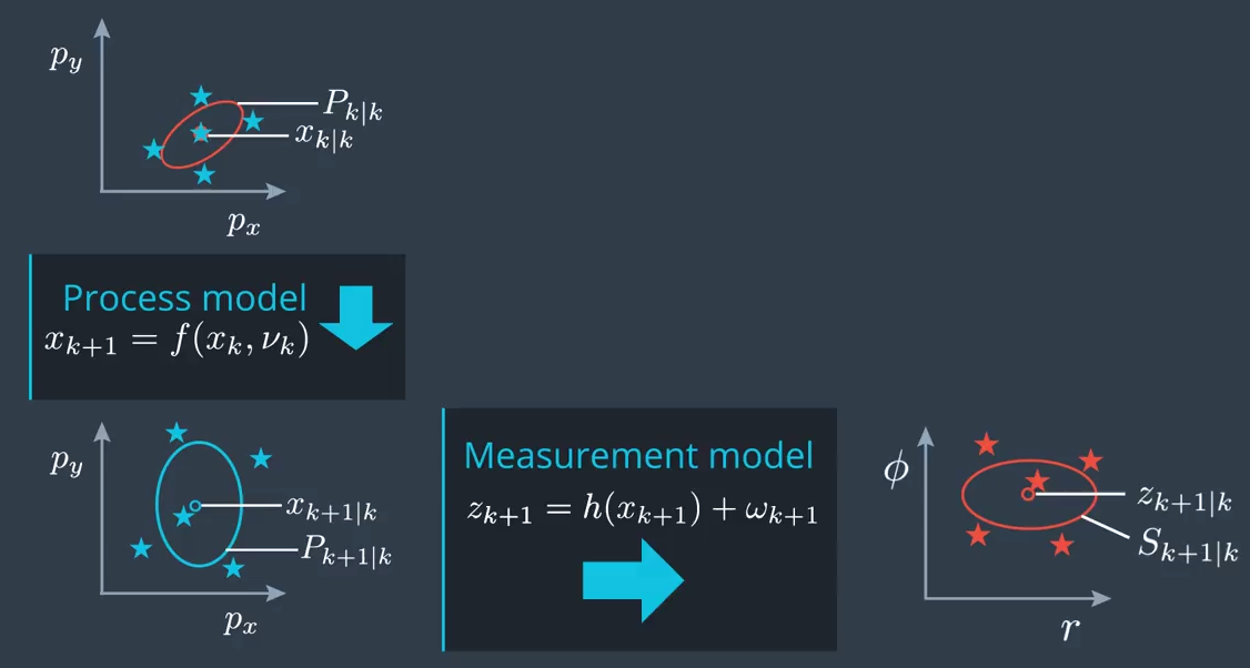
The prediction step of the unscented Kalman filter consists of
- Generating sigma points.
- Predicting the sigma points using the process model.
- Predict a mean state and covariance matrix from the sigma points.
These steps are summarized in the following figure and explained in more detail in the next sections.
Generate Sigma Points
We start with the posterior, the state $x_{k|k}$ and its covariance $P_{k|k}$ from the previous iteration. They represent the distribution of our current state. For this distribution we want to generate sigma points. The number of sigma points depends on the state dimension \(n_x\) and is calculated according to
\[n_{\sigma} = 2 n_x + 1\]Assuming a state dimesion of $n_x = 5$, this results in $n_{sigma} = 11$. The first sigma point is the mean of the state. This leafs us with $2 n_x$ sigma points for each state dimension, which will be spread in different directions.
The sigma points are stored in the following matrix
\[\mathcal{X}_{k \vert k} = \begin{bmatrix} \star & \star & \star & \star & \star & \star & \star & \star & \star & \star & \star \end{bmatrix}\]where each column of this matrix represents a sigma point. The rule how to generate sigma points is shown in the next equation:
\[\begin{equation} \mathcal{X}_{k|k} = \begin{bmatrix} x_{k|k} & x_{k|k} + \sqrt{(\lambda + n_x) P_{k|k}} && x_{k|k} - \sqrt{(\lambda + n_x) P_{k|k}} &\\ \star & \star \star \star \star \star && \star \star \star \star \star &\\ \end{bmatrix} \label{eq:X_sig} \end{equation}\]where $\lambda$ is a design parameter that lets one decide where in relation to the error ellipse the sigma points should be placed. A good rule of thumb is
\[\lambda = 3 - n_x\]The square root of a matrix can be found by several algorithms using the following relation:
\[A = \sqrt(P_{k|k}) \Leftarrow A^{T}A = P_{k|k}\]The first column of the matrix in equation \ref{eq:X_sig} tells us what the first sigma point is. This first sigma point corresponds to the means state estimate. The next term in the matrix $x_{k|k} + \sqrt{(\lambda + n_x) P_{k|k}}$ contains five more sigma points in the previous example. These sigma points are placed around the error “ellipse” (in 2D) and scaled by lambda. If lambda is large the sigma points move further away from the mean state. Otherwise, if lambda is small the sigma points move closer to the mean state. This all happens in relation to the error ellipse.
The final term in the matrix given in \ref{eq:X_sig} are the same vectors but in the opposite direction because of the minus sign.
UKF Augmentation
When using the unscented Kalman filter the underlying process model is usually nonlinear.
\[x_{k+1} = f(x_k, \nu_k)\]To account for the process noise $\nu_k$, the state vector can be augmented but first a note on the process noise.
It is important to distinguish between the noise vector itself and the vector that acts on the process model. The noise vector itself is independent of the process model, doesn’t express the effect on the state vector and is independent of $\delta t$.
The covariance matrix $Q$ of the process noise vector is
\[Q = E\{ \nu_k \nu_k^T \}\]and contains the variances of the proces noise vector on the diagonal. On the offdiagonal are the covariances but these are normally uncorrelated and therefore zero. This is because the process noises are often considered independent of each other. If this is not the case the entries shoudl be given an appropriate value, which is a parameter that should be tuned.
To represent the uncertainty of the covariance matrix $Q$ with sigma points, the previously mentioned augmentation can be used. Therefore, the the state vector $x$ is agumented by the noise vector $\nu$, which results in a new state vector $x_{aug}$ with dimension $n_{aug} = n_x + n_{\nu}$. This augmentation also results in $n_{\sigma} = 2 n_{aug} + 1$ sigma points. In the example above we get $15$ sigma points when we assume a dimension of two for the noise vector. The additional sigma points will be representing the uncertainty caused by the process noise.
To get the augmented matrix containing the sigma points we also need the augmented covariance matrix $P_{aug}$, which has seven rows and columns using the same example. It has an additional lower right block which contains the matrix $Q$ of the process noise.
\[P_{aug,k|k} = \begin{bmatrix} P_{k|k} & 0 \\ 0 & Q \end{bmatrix}\]Finally the augmented matrix is calculated according to
\[\mathcal{X}_{k|k} = \begin{bmatrix} x_{aug,k|k} & x_{aug,k|k} + \sqrt{ (\lambda + n_{aug}) P_{aug,k|k} } && x_{aug,k|k} - \sqrt{ (\lambda + n_{aug}) P_{aug,k|k} } & \end{bmatrix}\]with scaling factor $\lambda = 3 - n_{aug}$.
Predict Sigma Points
For the prediction step of the unscented Kalman filter, the sigma points of \(\mathcal{X}_{k \vert k} \in \mathbb{R}^{n_{aug} \times n_{sigma}}\) are inserted into the process model
\[\mathcal{X}_{k+1|k} = f(x_k,\nu_k)\]The input to the model has dimension $n_{aug}$, whereas the output has dimension $n_x$. This means that the matrix with the predicted sigma points has dimension of $n_x \times n_{\sigma}$.
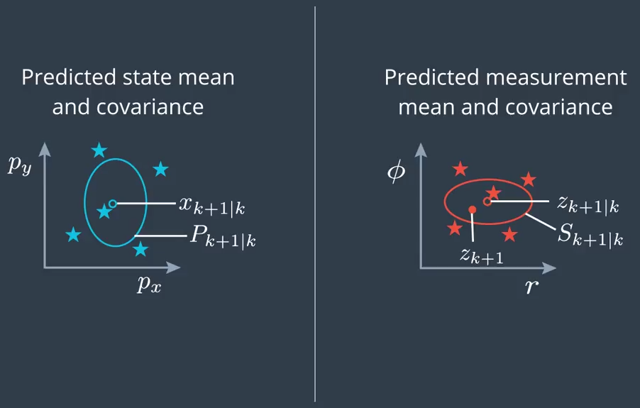
Predict Mean and Covariance
The predicted sigma points are used to calculate a predicted mean and covariance matrix.
The standard rule for calculating the mean and covariance of a group of state samples is given by the following equations
\[\begin{align} x_{k+1|k} &= \sum_{i=1}^{n_{aug}} \omega_i \mathcal{X}_{k+1|k,i} \\ P_{k+1|k} &= \sum_{i=1}^{n_{aug}} \omega_i (\mathcal{X}_{k+1|k,i} - x_{k+1|k})(\mathcal{X}_{k+1|k,i} - x_{k+1|k})^T \end{align}\]where $\omega_i$ are used to weight every sigma point. These weights depend on the spreading parameter $\lambda$ and are calculated according to
\[\begin{align} \omega_i &= \frac{\lambda}{\lambda + n_{aug}}, && i = 0 \\ \omega_i &= \frac{\lambda}{2(\lambda + n_{aug})}, && i = 2 \ldots n_{aug} \end{align}\]$\lambda$ was used before to set how far we want to spread the sigma points. Before we had a covariance matrix and generated sigma points. Now we are doing the inverse step. We have predicted sigma points and we want to recover the covariance matrix. Therefore, we also have to invert the spreading of the sigma points, which is what the weights do. The literature provides several ways to define these weights.
Update
In the update step, first we predict the measurement mean $z_{k+1 \vert k}$ and its covariance $S_{k+1 \vert k}$ from the previously predicted state $x_{k+1 \vert k}$. The final step is to incorporate the sensor measurement $z_{k+1}$. These two steps are shown in the following figure.
Predict Measurement
Transform the predicted state into the measurement space which is done by the measurement model.
\[z_{k+1} = h(x_{k+1}) + \omega_{k+1}\]It is important to consider which kind of sensor produced the measurement, e.g. radar or laser and use the corresponding measurement model.
The problem here of transforming a distribution through a nonlinear function is similar to that in the prediction step. This allows us to apply exactly the same unscented transformation approach as before during the state prediction. However, we don’t have to generate sigma points again, since wea already have them from the prediction step. Furthermore, the agumentation is not necessary in this case. In the prediction step, the augmentation was necessary because the process model had a nonlinear effect on the state. Assuming a radar measurement, the radar measurement is a nonlinear function but the the measurement noise acts has a purely additive effect. There is an easier way instead of augmenting the predicted state vector again, which we will see soon.
All that is left to do is to transform the individual sigma points we already have predicted in to the measurement space. Then use them to calculate the measurement mean $z_{k+1|k}$ and the covariance $S_{k+1|k}$ of the predicted measurement.
Again we want to store the transformed sigma points as columns of the following matrix
\[\mathcal{Z}_{k+1|k} = \begin{bmatrix} \star & \star & \star & \star & \star & \star & \star & \star & \star & \star & \star \end{bmatrix}\]This matrix has dimension $n_z \times n_{sigma}$ and it is obtained using the measurement model $z_{k+1} = h(x_{k+1}) + \omega_{k+1}$ and setting the measurement noise $\omega_{k+1}$ to zero for now.
Now to calculate the mean and covariance matrix from these sigma points, similar equations as before in the prediction step are utilized.
\[\begin{align} z_{k+1|k} &= \sum_{i=1}^{n_{aug}} \omega_i \mathcal{Z}_{k+1|k,i} \\ S_{k+1|k} &= \sum_{i=1}^{n_{aug}} \omega_i (\mathcal{Z}_{k+1|k,i} - z_{k+1|k})(\mathcal{Z}_{k+1|k,i} - z_{k+1|k})^T + R \end{align}\]Additonaly, the measurement noise covariance $R$ is added to calculate the measurement covariance matrix $S$. Instead of the augmentation it is possible to just add $R$ because the masurement noise $\omega_k$ does not has a nonlinear effect on the measurment but is purely additiv.
\[R = E\{\omega_k \omega_k^T\}\]Update State
To update the state mean and its covariance matrix with the measurement we utilize.
- the predicted state mean $x_{k+1 \vert k}$ and its covariance $P_{k+1 \vert k}$
- the predicted state measurement mean $z_{k+1 \vert k}$ and its covariance $S_{k+1 \vert k}$
We have both of these informaiton available in additon to the actual sensor measurement $z_{k+1}$. In the prediciton step we only needed the time of when the measurement was received. Now in the update step, we actually need the measurement values itself and the sensor type. The sensor type tells us which measurement model to use.
Processing Chain
The update step closes the processing chain and in the following the steps to update the state mean and its covariance are sumarized.
Updated state mean
\[x_{k+1|k+1} = x_{k+1|k} + K_{k+1|k}(z_{k+1} - z_{k+1|k})\]Covariance matrix update
\[P_{k+1|k+1} = P_{k+1|k} - K_{k+1|k}S_{k+1|k}K_{k+1|k}^{T}\]These two steps are exactly the same for the extended Kalman filter. The only difference is how the Kalman gain is calcualted. To calculate it we need the cross-correlation between sigma points in state space and measurement space
Kalman Gain
\[K_{k+1|k} = T_{k+1|k}S_{k+1|k}^{-1}\]Cross-correlation
\[T_{k+1|k} = \sum_{i=0}^{2n_{aug}} \omega_i (\mathcal{X}_{k+1|k,i} - x_{k+1|k}) (\mathcal{Z}_{k+1|k,i} - z_{k+1|k})^{T}\]References
A useful resource to learn more about state estimation is the Udacity self driving car Nanodegree


Comments