CTRV Model

Introduction

The constant turn rate and constant velocity model (in short CTRV) is used to model vehicles. Using the function $x_{k \vert k} = f(x_k, \nu_k)$ the model predicts the new state $x_{k \vert k}$ of the vehicle at time $k+1$ from the state $x_{k}$ and the noise vector $\nu_k$ at the current time step $k$. In addition to a constant velocity the model assumes also a constant turn rate which makes it more accurate than the constant velocity model, especially in curves.

The CTRV Model (Source: Udacity self driving car ND)

State Vector and Process Model

The state vector of the ctrv model is given as

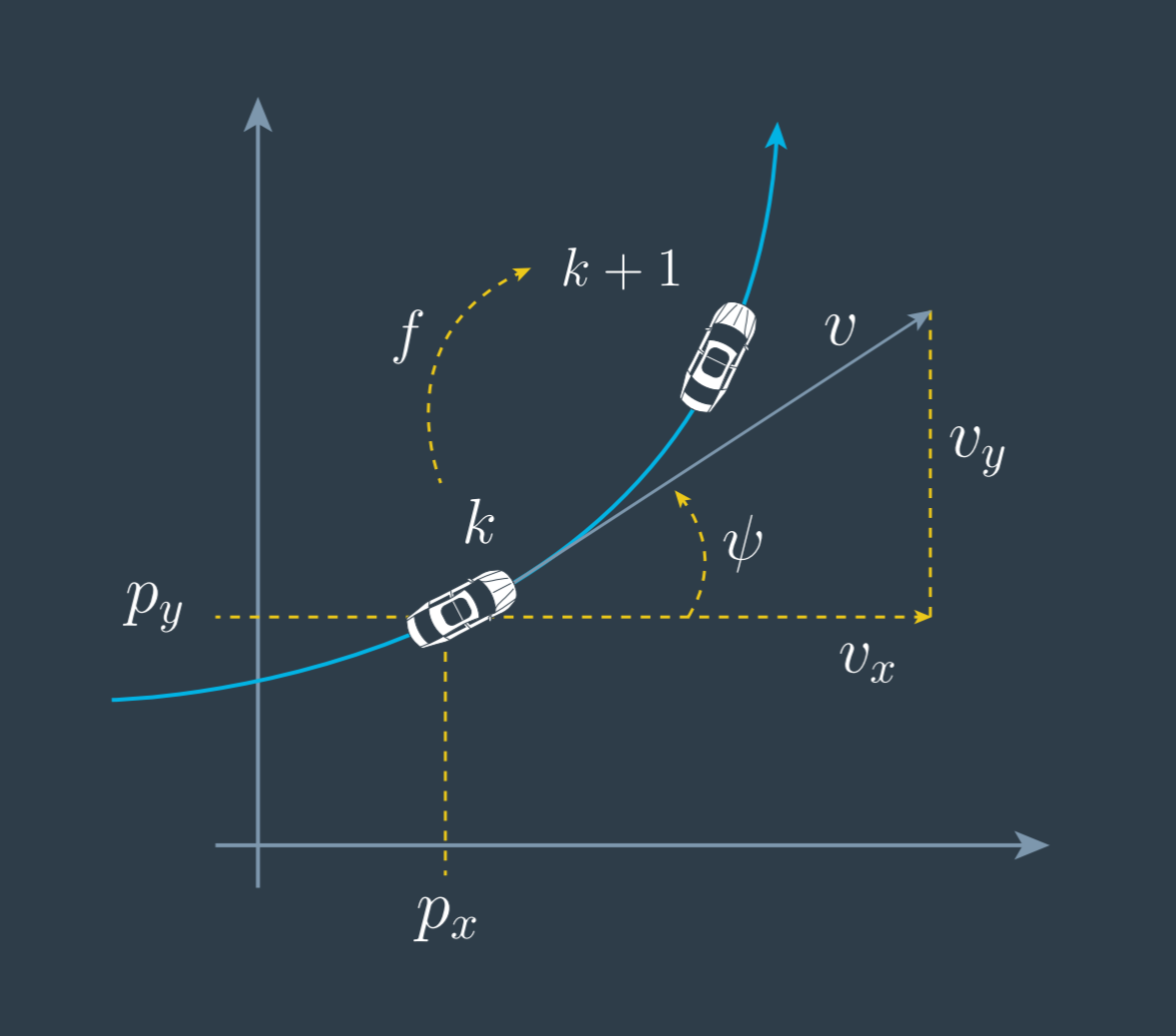
\[x = \begin{bmatrix} p_x & p_y & v & \psi & \dot \psi \end{bmatrix}^T\]

To derive the process model we investigate in the change rate of the state $x$, which is called $\dot{x}$. From the geometric relations, shown in the image above, we find how the change rate $\dot{x}$ depends on the state $x$, which is a differential equation $\dot{x} = g(x)$. To derive this differential equation the goal is to express the five time derivatives of the state, in dependency of any of the state elements.

\[\dot{x} = \begin{bmatrix} \dot{p}_x \\ \dot{p}_y \\ \dot{v} \\ \dot{\psi} \\ \ddot{\psi} \end{bmatrix} = \begin{bmatrix} v \cdot \cos{\psi} \\ v \cdot \cos{\psi} \\ 0 \\ \dot{\psi} \\ 0 \end{bmatrix}\]

Obviously the change in velocity and turn rate is zero because this is the underlying assumption of the ctrv model. A constant velocity $v$ and a constant turn rate $\dot{\psi}$ is not changing. Put in mathematical terms, the derivative of a constants is zero.

Discrete State Prediction

The discrete time step $k$ relates to the continuous time value $t_k$. To get from the discrete time step $k := t_k$ to $k+1 := t_{k+1}$ we make use of the time difference $\Delta t = t_{k+1} - t_{k}$ and integrate the change rate $\dot{x}$ of the state $x$ over this time period. The result of this integral is added to the current state $x_k$.

\[x_{k+1} = x_k + \int_{t_k}^{t_{k+1}} \begin{bmatrix} \dot{p}_x \\ \dot{p}_y \\ \dot{v} \\ \dot{\psi} \\ \ddot{\psi} \end{bmatrix} \mathrm{d} t\]

To solve this integral, every row of the change rate vector can be integrated.

\[\begin{align} \int_{t_k}^{t_{k+1}} \begin{bmatrix} \dot{p}_x \\ \dot{p}_y \\ \dot{v} \\ \dot{\psi} \\ \ddot{\psi} \end{bmatrix} \mathrm{d} t &= \begin{bmatrix} \int_{t_k}^{t_{k+1}} \dot{p}_x \mathrm{d} t \\ \int_{t_k}^{t_{k+1}} \dot{p}_y \mathrm{d} t \\ \int_{t_k}^{t_{k+1}} \dot{v} \mathrm{d} t \\ \int_{t_k}^{t_{k+1}} \dot{\psi} \mathrm{d} t \\ \int_{t_k}^{t_{k+1}} \ddot{\psi} \mathrm{d} t \\ \end{bmatrix} = \begin{bmatrix} \int_{t_k}^{t_{k+1}} v \cdot \cos{\psi} \mathrm{d} t \\ \int_{t_k}^{t_{k+1}} v \cdot \sin{\psi} \mathrm{d} t \\ \int_{t_k}^{t_{k+1}} \dot{v} \mathrm{d} t \\ \int_{t_k}^{t_{k+1}} \dot{\psi} \mathrm{d} t \\ \int_{t_k}^{t_{k+1}} \ddot{\psi} \mathrm{d} t \\ \end{bmatrix} \\ &= \begin{bmatrix} \int_{t_k}^{t_{k+1}} v \cdot \cos{\psi} \mathrm{d} t \\ \int_{t_k}^{t_{k+1}} v \cdot \sin{\psi} \mathrm{d} t \\ \int_{t_k}^{t_{k+1}} 0 \mathrm{d} t \\ \int_{t_k}^{t_{k+1}} \dot{\psi} \mathrm{d} t \\ \int_{t_k}^{t_{k+1}} 0 \mathrm{d} t \\ \end{bmatrix} = \begin{bmatrix} \int_{t_k}^{t_{k+1}} v \cdot \cos{\psi} \mathrm{d} t \\ \int_{t_k}^{t_{k+1}} v \cdot \sin{\psi} \mathrm{d} t \\ 0 \\ \int_{t_k}^{t_{k+1}} \dot{\psi} \mathrm{d} t \\ 0 \\ \end{bmatrix} \end{align}\]