Model predictive control reframes the task of following a vehicle into an optimization problem. The solution to this optimization is a time ordered set of optimal actuator inpus for steering $\delta$ and acceleration $a$, which can be positive or negative. When these inputs are integrated using an initial state and the underlying vehicle model, the result is an optimal trajectory. A trajectory is a time ordered set of vehicle states. To find this optimal trajectory, a cost function is utilized, which also accounts for the vehicle constraints. The problem of following a reference trajectory can be solved by minimizing the distance to this reference. Therefore, the actuator inputs are optimized during each step in time in order to minimize the cost of the predicted trajectory. Once the optimal trajectory is found, only the first set of actuation commands is applied to the vehicle. The rest of the optimized trajectory is ignored because the sourrounding environment could have been changed already and the underlying model is only approximate. In the next time step the process, to calculate a new optimal trajectory over a finite horizon is repeated with the new initial state. That is why this method is also known as receding horizon control.
Cost function
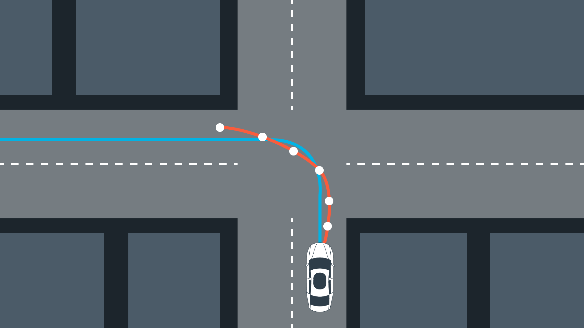
To design a cost function we think about the reference which provides the desired position an orientation of the vehicle. Provided that we have a given reference path. A high cost will occur when the vehicle is far away from the center lane and has a different heading. Therefore, the cross track error (cte) and the orientation error are used in the cost function:
1
2
3
4
5
double cost = 0;
for (int t = 0; t < N; t++) {
    cost += pow(cte[t], 2);
    cost += pow(epsi[t], 2);
}
One problem with this cost function is that the vehicle might just stop to avoid increasing costs. The mentioned cost function also does not incorporate the vehicle constraints, which can lead to drastically changing actuator inputs and may damage the actuators.
Avoid Stopping
To deal with stopping along the way, a desired reference velocity can help to overcome this issue. The cost function will penalize the vehilce for not maintaining that reference velocity.
1
2
cost += pow(v[t] - 50, 2);
cost += pow(dist[t], 2);
Another option is to measure the eclidean distance between the vehicle’s current and the goal position and then add that distance to the cost.
Additional Costs
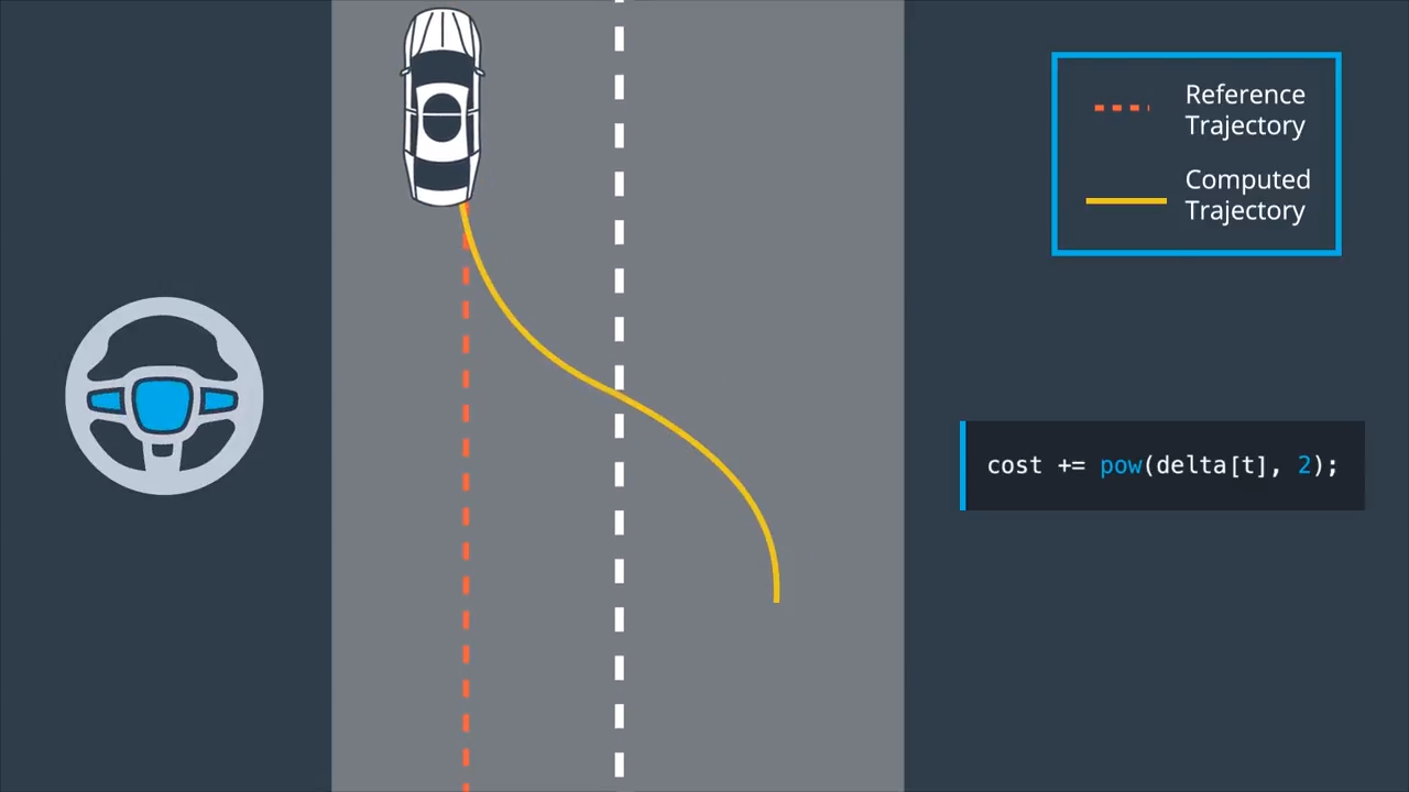
To account for the mentioned actuator limits the cost function can also be used to incorporate the inputs. This can be used to penalize the magnitude of the inputs as well as the change rates. If we want to change lanes we would have a large cross-track error, due to an offset to the reference. However, we want to penalize turning the steering wheel sharply, which will yield a smoother lane change.
The control input magnitude can be added to the cost in the following way:
1
cost += pow(delta[t], 2);
To capture the change rate of the control input in order to add some termporal smoothness, we add the following to the cost function:
1
2
3
for (int t = 0; t < N; t++) {
    cost += pow(delta[t+1] - delta[t], 2);
}
This term captures the difference between the next control input and the current one. This reduces the change rate and gives us further control over the inputs.
Hyperparameters
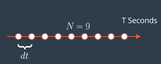
Model predictive control allows to choose the number of optimization steps $N$. Another tuning parameter is the sampling rate or the time in between the timesteps $dt$, which defines how much time elapsed between actuations. The product of these two parameters results in the prediction horizon $T$, which is the duration over which future predictions are made. In the case of a self driving vehicle the duration of this horizon should be a few seconds because the environment keeps changing. Long horizons increase the computation costs and do not provide more safety because the environment won’t stay the same in the near future.
Horizon Length
The number of optimization steps determins the size of the control input vector $[\delta_1, a_1, \delta_2, a_2, \dots, \delta_{N-1}, a_{N-1}]$. Integrating this vector using the vehicle model results in an optimal trajectory, found by minimizing a cost function. Increasing the horizon results in higher computational costs.
Timestep Duration
For a computers continuous trajectories need to be discretized. The step size of these discretizations is $dt$. Large values of $dt$ result in a high discretization errors. To accurately represent a continous trajectory $dt$ should be small. On the other hand, low values increase the computation and are not always necessary. A lower limit depends on the rate new measurements are received.
To find parameters for $N$ and $dt$ is to define a resonable $T$ and think about the consequences of the two parameters.
MPC Algorithm
To setup the mpc algorithm it is necessary to define the previously mentioned time horizon $T$, which specifies the duration of the trajectory. This is done by choosing $N$ and $dt$. Since, mpc is based on a vehicle model, a dynamic or kinematic model has to be chosen. Model predictive control, tries to reduce the cross-track error to a reference path. Therefore the cte and orientation errors are also included in the model:
\[\label{model} \begin{align} \begin{split} x_{t+1} &= x_{t} + v_{t} \cos(\psi_{t}) dt \\ y_{t+1} &= y_{t} + v_{t} \sin(\psi_{t}) dt \\ \psi_{t+1} &= \psi_{t} + \frac{v_{t}}{L_f} \delta_{t} dt \\ v_{t+1} &= v_{t} + a_{t} dt \\ cte_{t+1} &= f(x_{t}) - y_{t} + v_{t} \sin(e\psi_{t}) dt \\ e\psi_{t+1} &= \psi_{t} - \psi_{des,t} + \frac{v_{t}}{L_f} \delta_{t} dt \\ \end{split} \end{align}\]The constraints of an optimization problem are used to limit the actuator values.
\[\begin{align} \delta &\in [-25^{\circ}, 25^{\circ}] \\ a &\in [-1, 1] \end{align}\]To obtain an optimal trajectory a cost function like the following can be minimized:
\[\label{cost} J = \sum_{t=1}^{N} cte_{t}^2 + e\psi_{t}^2\]After setting up the requirements for an optimization solver, the feedback loop is executed in the following way:
- Pass initial state $[x_1, y_1, \psi_1, v_1, cte_1, e\psi_1]$ to the model predictive controller
- Call the optimization solver
- Solver finds optimal control inputs \ref{inputs} that minimizes the cost function \ref{cost}
Latency
The time it takes for a command to adjust the actuator and until the actuator reaches its final position is known as latency. This time needs to be taken into consideration while solving for the optimal actuator inputs.


Comments