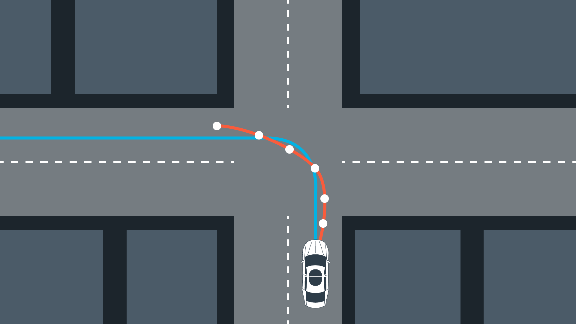
Path Planning

Path planning generates vehicle trajectories using fused sensor data to understand the environment around the vehicle, and localization data to determine where car is located in that environment.

The path planning unit uses this data to decide where to drive next by generating a trajectory. This trajectory is passed to the controller to steer the vehicle.

The following sections summarize the foundations of

• Search algorithms used in discrete path planning
• Prediction which uses the data from sensor fusion to predict where surrounding objects are likely to do.
• Behavior planning where a decision for the vehicle in the next 10 seconds is made.
• Trajectory generation where smooth, drivable and collision-free trajectories are generated for the motion controller to follow.

A vehicle will be able to avoid collisions, maintain safe distances between other traffic and pass other vehicles to reach its target faster.

Search

A Star

A* is a discrete search algorithm that uses a heuristic function $h$ to find a goal state starting from an initial start state. The heuristic function $h(x,y) \leq \text{distance to goal from x, y}$ can be the number of steps it takes to the goal if no obstacles were inside a grid. Another commonly used heuristic function is the euclidean distance from start to goal. In A* the node with the lowest $f$ value is expanded, where $f = g + h(x,y)$. The function $g$ is the cost for reaching the current node, which can be the number of steps it took to get to this node from the start.

Wikipedia A star

Dynamic Programming

Dynamic programming finds a shortest path from any starting location to one or more goal states. Therefore, this method is not limited to a single starting location. In reality the environment is stochastic, then the outcome of actions is non deterministic. This means that the vehicle can find itself anywhere in the map, which requires a plan for more than just a single position. Dynamic programming finds a plan for any position.

Given:

• Map
• One or more goal positions

Output:

• Best path from any possible starting location

Dynamic programming uses a policy, which is a function that maps a grid cell or a state into an action $a = p(x,y)$. Action can be a movement for example.

A value function associates to each grid cell the length of the shortest path to the goal. This function is zero for the goal and one for each adjacent state to the goal. All values are recursively calculated by taking the optimal neighbor $x’, y’$ and its value $f(x’, y’)$ and by adding the cost it takes to get there, which is one in the following example.

\[f(x,y) = \min_{x', y'} f(x', y') + 1\]

With this value function, the optimal control action is obtained by minimizing the value, which is a hill climbing type of action.

Robot Motion Planning Problem

Given:

• Map
• Starting location
• Goal location
• Cost

Goal: Find minimum cost path

double cost = 0;
for (int t = 0; t < N; t++) {
    cost += pow(cte[t], 2);
    cost += pow(epsi[t], 2);
}

One problem with this cost function is that the vehicle might just stop to avoid increasing costs. The mentioned cost function also does not incorporate the vehicle constraints, which can lead to drastically changing actuator inputs and may damage the actuators.

Prediction

To deal with stopping along the way, a desired reference velocity can help to overcome this issue. The cost function will penalize the vehilce for not maintaining that reference velocity.

cost += pow(v[t] - 50, 2);
cost += pow(dist[t], 2);

Another option is to measure the eclidean distance between the vehicle’s current and the goal position and then add that distance to the cost.

Behavior Planning

Actuator constraints (Source: Udacity self driving car ND)

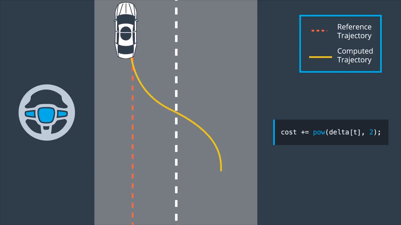
To account for the mentioned actuator limits the cost function can also be used to incorporate the inputs. This can be used to penalize the magnitude of the inputs as well as the change rates. If we want to change lanes we would have a large cross-track error, due to an offset to the reference. However, we want to penalize turning the steering wheel sharply, which will yield a smoother lane change.

The control input magnitude can be added to the cost in the following way:

cost += pow(delta[t], 2);

To capture the change rate of the control input in order to add some termporal smoothness, we add the following to the cost function:

for (int t = 0; t < N; t++) {
    cost += pow(delta[t+1] - delta[t], 2);
}

This term captures the difference between the next control input and the current one. This reduces the change rate and gives us further control over the inputs.

Trajectory Generation

Model predictive control allows to choose the number of optimization steps $N$. Another tuning parameter is the sampling rate or the time in between the timesteps $dt$, which defines how much time elapsed between actuations. The product of these two parameters results in the prediction horizon $T$, which is the duration over which future predictions are made. In the case of a self driving vehicle the duration of this horizon should be a few seconds because the environment keeps changing. Long horizons increase the computation costs and do not provide more safety because the environment won’t stay the same in the near future.

Time steps and horizon length (Source: Udacity self driving car ND)

\[\label{inputs} \begin{bmatrix} \delta_1 & a_1 \\ \delta_2 & a_2 \\ \vdots & \vdots \\ \delta_{N-1} & a_{N-1} \\ \end{bmatrix}\]

Latency

The time it takes for a command to adjust the actuator and until the actuator reaches its final position is known as latency. This time needs to be taken into consideration while solving for the optimal actuator inputs.

Additional reading

• PID Controller
• Controller